How to Perform a Kruskal-Wallis test in Julius
This article will provide a comprehensive review on how to perform a Kruskal-Wallis test in Julius.
Introduction
When discussing data, you may have encountered the terms “parametric” and “non-parametric” methods.These terms are used in statistics to describe the various types of statistical tests and methods based on the assumptions of the data.
Parametric methods rely on specific assumptions about the population distribution from which the data was obtained. The assumptions typically include:
1. Data must be normally distributed.
2. The variances of the population must be equal.
3. Observations must be independent of each other.
In contrast, non-parametric methods do not rely on the dataset being normally distributed. These methods are more flexible than their parametric counterparts. While non-parametric methods are often less powerful, they are more versatile and robust, making them suitable for a wider range of data types and distribution. They are especially useful for handling datasets that are ordinal, do not follow normal distribution, or have relatively small sample sizes.
Usually, when the assumptions of a parametric test are violated, the best practice is to use the equivalent non-parametric test. Below is a quick guide showing common parametric tests along with their non-parametric equivalents:
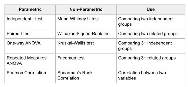
The type of non-parametric test we are focusing on in this use case is the Kruskal-Wallis test.
Dataset Overview
The dataset we will use is from Rdatasets, a repository of datasets that are distributed in R packages. The file is called Spruce, which I have modified to fit the purpose of our analysis. This dataset tracks the growth of spruce trees under four different treatments (originally plot location, but changed to treatment for this use case). Below is a snapshot of the dataset that we will use.
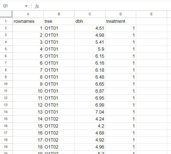
The dataset contains four columns: rownames, tree, dbh, and treatment. DBH stands for ‘diameter at breast height’ and is a common metric used to estimate tree growth (henceforth referred to as dbh). For this use case, we can assume it was calculated in inches. For treatment, we have four separate conditions:
1. Control
2. 10% perlite
3. 50% perlite
4. Sheep manure
We want to see if treatment affects the growth rate of spruce trees. Since we have four different treatments to compare, we need a method that allows for this comparison. Our options are the One-way ANOVA or Kruskal-Wallis test. The normality test will determine which test we use.
Step-by-Step Walkthrough
Step 1: Import your dataset into Julius
This walkthrough will be done using Python; however, you can also perform the analysis in Julius using R by switching the code runtime environment toggle in the top right of the chat interface.
To connect a dataset, you can either select the paperclip icon in the input bar to upload your data as a file, or you can also paste in a link to a publicly-shared Google Sheet. In this case, we are going to connect to a Google Sheet containing the tree, treatment and identification information.
Prompt: “Please preview the dataset from Google Sheets.”
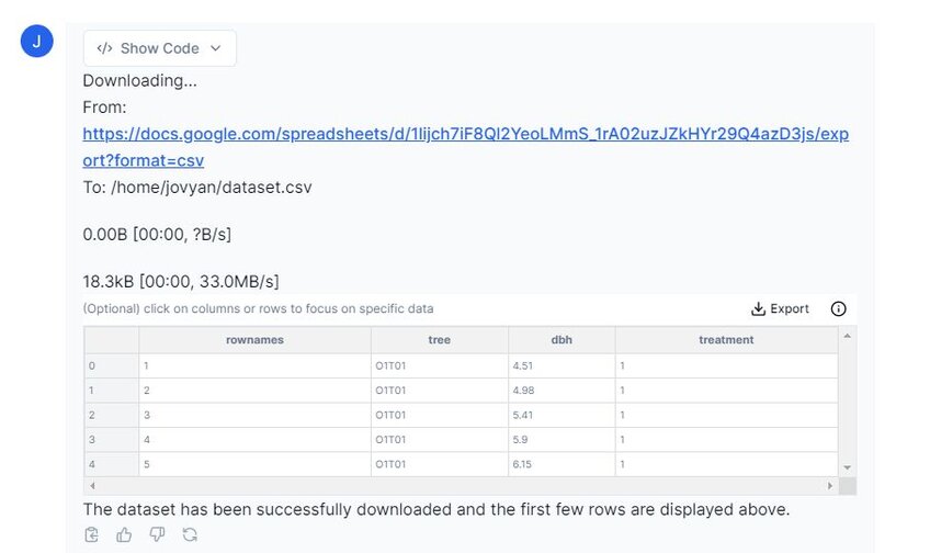
Above you can see that Julius has imported our dataset. This dataset has been previously examined for any missing or ‘null’ values, but please remember to do so with your own dataset before continuing with any analysis.
Step 2: Run Descriptive Statistics
Let’s prompt Julius to perform descriptive statistics on this dataset. Since we have four separate treatments, we must analyze each group individually. We are only going to work with the ‘dbh’ and ‘treatment’ columns, which we can specify to Julius by highlighting them in the chat by clicking on them.
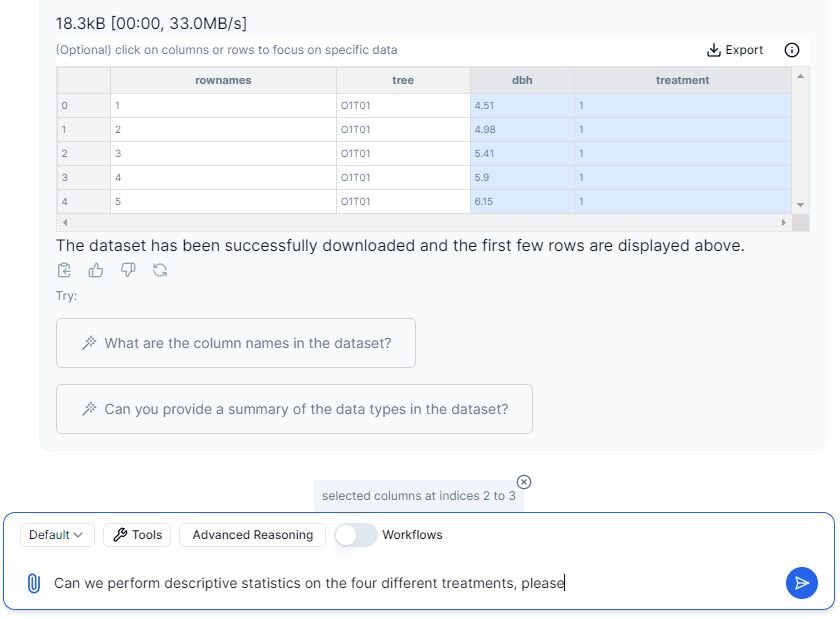
We can now continue with the prompt, as we have highlighted the designated columns.
Prompt: “Can we perform descriptive statistics on the four different treatments, please?”
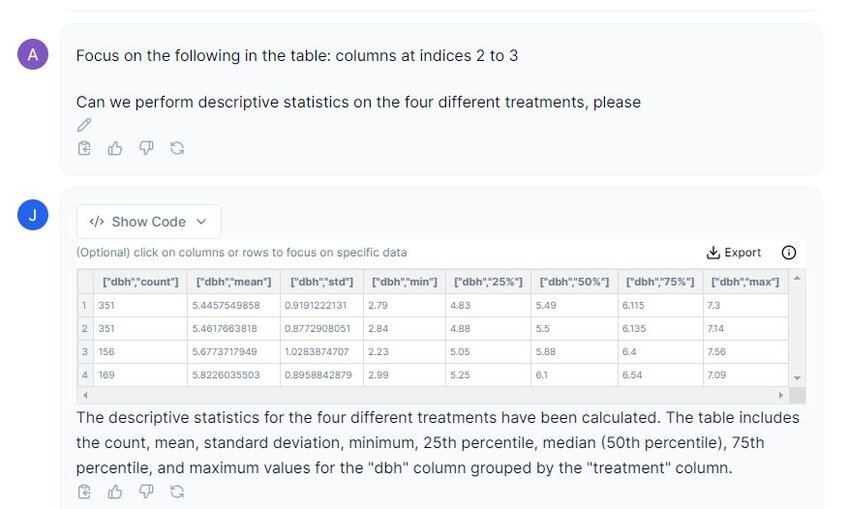
In the image above, we can see that Julius has given us a nice output of the descriptive statistics, including the count, mean, standard deviation, minimum and maximum values, as well as the 25%, 50% and 75% interquartile range. The sample sizes for each treatment are unequal indicated by the ‘count’ column/ This is important to note for some analyses as this may affect the type of tests you can use.
Step 3: Testing Assumptions
Our next step is to examine the assumptions that are required for the Kruskal-Wallis test. They are as follows:
1. Samples from each group must be independent from each other.
2. Data within each group can be ranked.
3. Variances must be homogenous.
4. Data should be obtained via random sampling.
We can assume random sampling and independence amongst samples for this use case. We need to test for homogeneity of variances and normality.
Let’s first take a look at normality for this dataset.
Prompt 1: “Can we create histograms to show the frequency of distribution of the dbh amongst the four treatments please?”
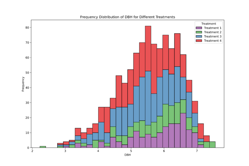
In the image above, Julius has plotted all four treatments onto one graph. The dataset appears to be skewed to the left. To confirm non-normally distributed, we can perform a normality test.
Prompt 2: “Please perform a normality test on each treatment.”
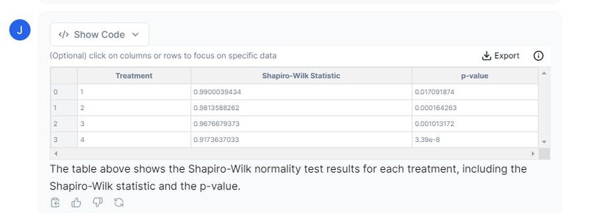
From the table displayed above, we can conclude that our data is non-normally distributed. We must continue with non-parametric methods.
Let’s take a look at the homogeneity of variances now to determine whether our dataset passes this assumption.
Prompt 3: “Please perform a homogeneity of variance test on this dataset.”
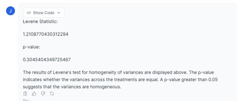
From the snapshot above, our dataset passes the assumption of homogenous variances (p ≥ 0.05). This means we can proceed with the Kruskal-Wallis test.
Step 4: Performing the Kruskal-Wallis test
Let’s perform the Kruskal Wallis test on our dataset.
Prompt: “Please perform the Kruskal-Wallis test on this dataset to determine if there are any differences between ‘treatment’ type and ‘dbh’.
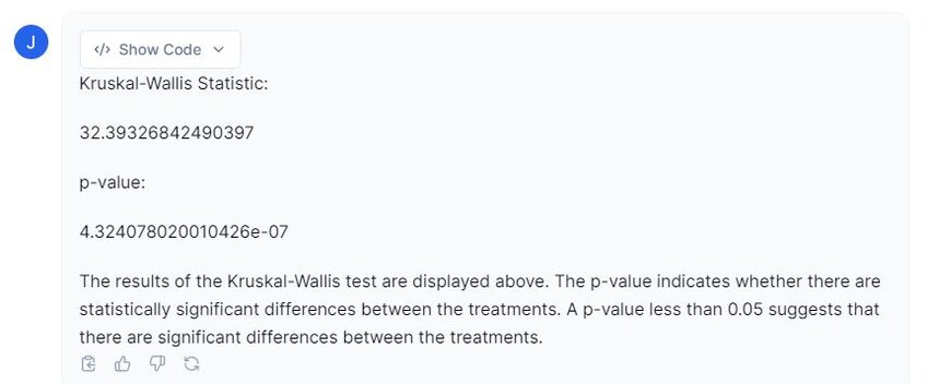
Examining the image above, Julius provides a Kruskal-Wallis test statistic of 32.39, and a p-value ≤ 0.001. However, this test does not show where the differences are located. We need post hoc tests to identify which treatments differ significantly.
Step 5: Performing Post Hoc Tests
We will use Dunn’s test with Bonferroni correction, which handles unequal sample sizes and controls for family-wise error rates.
Prompt: “Perform a Dunn’s post hoc test with Bonferroni correction on this dataset please.”
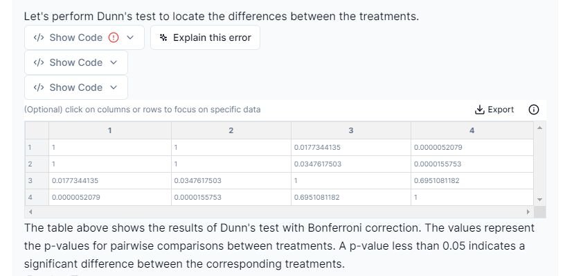
From the results above, we can conclude that the following treatments are statistically significant from one another:
1. Treatment 1 vs. Treatment 3: p-value = 0.0177
2. Treatment 1 vs. Treatment 4: p-value ≤ 0.001
3. Treatment 2 vs. Treatment 3: p-value = 0.0348
4. Treatment 2 vs. Treatment 4: p-value ≤ 0.001
Our final step is to create a visualization that effectively shows the findings from our analysis.
Step 6: Creating a Boxplot
We will use the ‘compact letter display’ (CLD) or ‘compact letter representation’ (CLR… not the bath cleaner) to show significance. The letters above the boxplots show significance: if they have the same letters, they are not significantly different; if they have different letters, they are statistically significant from one another.
Prompt: “Please create a boxplot of DBH by treatment.”

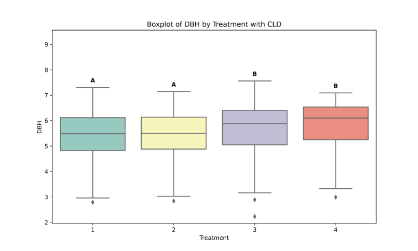
As depicted in the screenshot above, Julius has created a boxplot with CLD showing which treatments are statistically significant from one another.
Step 7: Reporting Results
Our final step is to report the results in a clear and concise manner:
“A Kruskal-Wallis H test was conducted to examine if there were any differences in spruce tree growth under four different treatments. The test revealed a statistically significant difference in diameter at breast height (DBH) between treatment groups, H(3) = 32.39, p ≤ 0.001.
Further post hoc tests revealed statistically significant differences between Treatment 1 and 3 (p = 0.017), Treatment 1 and 4 (p ≤ 0.001), Treatment 2 and 3 (p = 0.035) and Treatment 2 and 4 (p ≤ 0.001). No significant differences were found for any other treatment pairs.”
Conclusion
In this use case, we learned the difference between parametric and non-parametric tests, how to determine which method is suitable for our dataset, the assumptions required for the Kruskal-Wallis test, and how to interpret the results. Additionally, we discussed how to present our findings effectively and in a visually appealing manner. Julius guided us through this process seamlessly, making data analysis easy to understand.
