February 3rd, 2025
Paired T-Test Definition & Guide
By Connor Martin · 20 min read

You have a pair of sample datasets that are related to one another, such as before and after test scores for a class. You need a statistical method to determine what (if any) difference exists between those two related sets.
This is where the paired t-test comes in to help. It determines whether a significant difference exists between the two related data sets.
Key Takeaways
- A paired t-test is a statistical method used to identify significant differences between two related datasets, such as before-and-after measurements or data collected under two conditions for the same subject.
- The test requires dependent, continuous data with normally distributed differences to deliver reliable results.
- Paired t-tests are ideal for tracking changes over time, comparing treatment outcomes, or analyzing the effects of changes in processes or equipment.
What Is a Paired T-Test?
With a paired t-test, you start with a null hypothesis of 0, meaning you believe there is no difference between your two datasets. Your test then compares your sets of data. If the calculated difference deviates significantly from 0, you have enough evidence to reject the null hypothesis and conclude there is a statistically significant difference between your datasets.
Paired t-tests aren’t the only types of t-tests you have in your statistical arsenal. There are also two-sample t-tests – used when you have two independent groups that are unpaired and unrelated – and the one-sample t-test. With that latter test, you stack up the mean of a single sample to an already known value.
Key Assumptions of a Paired T-Test
You can only use a paired t-test confidently if your data meets a few assumptions. These assumptions include:
Normality of Differences
The differences between the paired measurements should follow an approximately normal distribution. This means the differences between paired measurements should be approximately symmetric and follow a bell-shaped curve when plotted, especially for smaller sample sizes.
Dependent Samples (Matched Pairs)
The two sets of measurements must come from matched pairs, not two independent samples. For example, they can be before-and-after measurements or data collected under two conditions for the same subject.
Paired samples must be related (e.g., measurements from the same individuals under different conditions) but should not influence one another.
Continuous Data
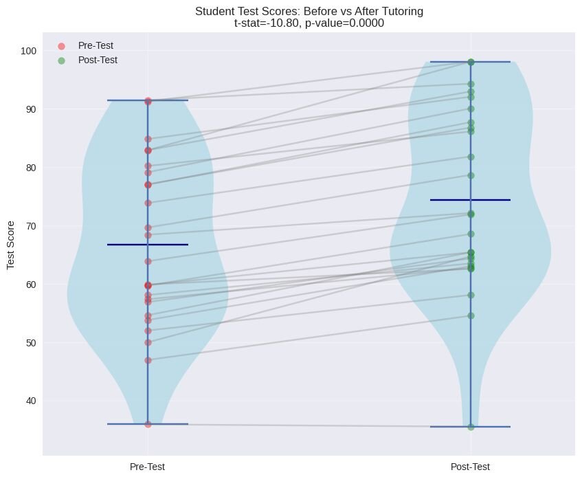
This test can only successfully analyze continuous data – discrete data is out of the picture because of the normal distribution requirement of a paired t-test. Weight, income, and height data all fall under the continuous umbrella, as do the student test scores we’ll be using in an example later.
When to Use a Paired T-Test
If you have paired datasets, you have the ingredients you need for your paired t-test recipe. Here are some solid potential application examples.
Practical Applications in Research and Business
Tracking changes over time is the stock-in-trade of a paired t-test, so it's no surprise that these tests have many applications in business and research.
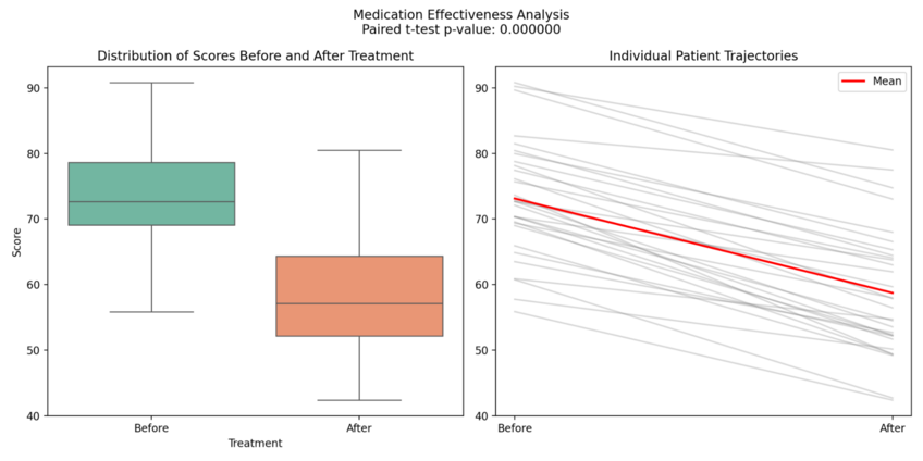
For research, consider studies conducted to determine how effective medication is on patients, with before-and-after figures showing the results. This would be perfect for a paired t-test.
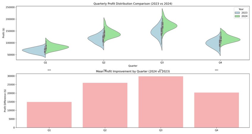
Business owners have all sorts of uses for this statistical test. Want to see what variance (if any) exists between profit and loss figures across two defined periods? A paired t-test shows you what you need to know. Manufacturing managers inside a business could also use this test to see if there’s any positive difference resulting from changes in their production cycles, such as the introduction of new machinery.

Examples of Common Scenarios
Versatility is the paired t-tests' biggest advantage. You likely already see that from the numerous examples of how you can use the test that we’ve already explained. And it’s that versatility that leads to the tests being used in the following common scenarios:
- Before-and-after measurements: You’ll get a taste of this in our manual example below. A paired t-test is excellent for measuring significant differences (assuming any exist) between what happens after introducing something new and what happened before.
- Comparing two treatments: Researchers can use these tests as part of their studies, especially when testing new medications. Get yourself a medicated group and a placebo group, and you have related datasets you can plug into a paired t-test.
- Testing equipment or methods: Want to check for consistency across two different versions of the same piece of equipment? The paired t-test is your answer. For instance, you might have a pair of thermometers (each made by different brands), and you want to see that they each deliver the same temperature readings where appropriate.
How to Perform a Paired T-Test in 5 Steps
As with most statistical tests, a paired t-test involves following some clear and defined steps to get the numbers you need.
Step 1 – Collect and Organize Data
Pairing up is your goal with the data collection phase. Any data you collect has to be related (or paired, as the name implies) with that data being aligned into a table with two columns for analysis. Think of a before and after chart – see our example below – and you’re on the right track.
Step 2 – Verify Assumptions
Normal distribution, continuous data, and a justified pairing. Those are the assumptions you need to make for a paired t-test.
Data that fails to meet these assumptions requires alternative tests, such as the Wilcoxon signed-rank test for non-normal data.
Step 3 – Calculate Differences Between Pairs
It’s time to start calculating. First, use subtraction to find the difference between the two values for each pair. With that data, you can find the mean and standard deviation figures that you’ll need to complete your paired t-test.
Step 4 – Compute the Test Statistic
We’ll share the formula for calculating your test statistic below. For now, just know that you need the mean difference and standard deviation figures from the last step to plug into that formula. You’ll get a number from that formula – which you stack against your null hypothesis of 0 – and will use that number to find your p-value.
Step 5 – Analyze and Interpret the Results
The p-value will tell you whether to reject or fail to reject the null hypothesis. You only need to compare the calculated p-value with your chosen significance level - typically 0.05.
A p-value less than your significance level means you can wave goodbye to your null hypothesis of 0. You’ve found a significant difference between your paired groups. Whether that’s a good or bad thing depends on the type of difference you were hoping to see.
Paired T-Test Formula and Calculations
So far, you’ve learned what the steps to performing a paired t-test look like. Now, let’s look at the formulas and calculations involved.
Formula Breakdown
The formula for the paired t-test is as follows:

Here’s the breakdown of this formula:

Manual Calculation Example
We’ll take you into the classroom to demonstrate how to run a paired t-test manually.
Let’s say you’re a teacher. You’re about to introduce a few new teaching methods to your class, and you want to see if those methods have a positive effect. So, you will track your students’ test scores before and after implementing the new methods – the perfect situation for a paired t-test.
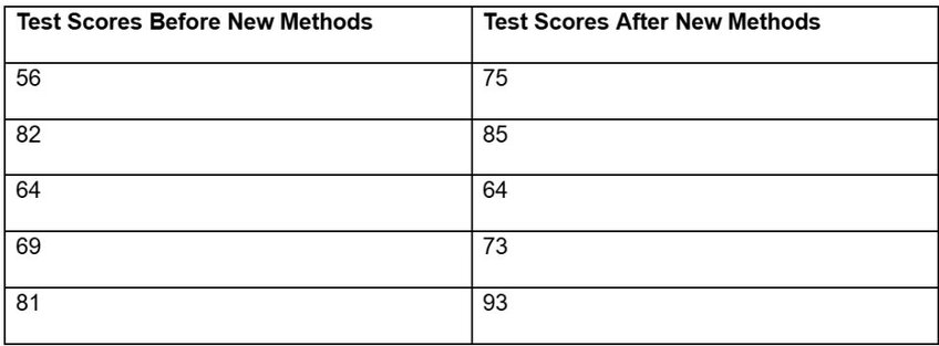
You do the tracking, and you end up with data that looks something like this:

Remember the formula we shared earlier?

We only have five students, so “n” is simple—it equals 5. Now, we need to calculate the mean of the differences between paired observations and then the standard deviation of the differences. Start by calculating 75 minus 56, and repeat for the other four students. You’ll get a total difference of 38, and the mean of those differences is 7.6.
Next, we calculate the standard deviation of the differences. You solve this by finding the mean, calculating the deviations from the mean, squaring the deviations, finding the variance, and then taking the square root of that formula. Following this process with our dataset returns a standard deviation of approximately 7.77
So, with all of those numbers, our t-statistic is 2.19. This indicates there is a substantial, positive difference in the test scores as a result of your new methods. (Congratulations!) You still need to compare that t-statistic to a p-value (likely found in a textbook or separate table), with the idea being that your t-statistic of 2.19 should show a low p-value, indicating there is good evidence against a null hypothesis of 0.
Using Statistical Software for Efficiency
Now, you can manually perform the paired t-test. However, statistical software is a far better option. It will be faster and more convenient, and the results will be more accurate. That’s not to mention all the advanced analyses you can perform using this tool.
How to Interpret Paired T-Test Results
Interpretation follows calculation with a paired t-test – a crucial set of steps that deliver meaning to the t-statistic you unveil.
P-Values and Statistical Significance
Remember that you start every paired t-test with the same null hypothesis – there is no significant difference between your two groups. That’s where p-values come into play.
Stacking your t-statistic against the relevant p-value shows if you have a confirmed null hypothesis or an alternative hypothesis showing a significant difference. The lower the p-value, the stronger the evidence against the null hypothesis.
Confidence Intervals and What They Mean
Confidence intervals give you a range of where the true result is likely to be. Let’s say you have a 95% confidence interval. That means you would expect your results to fall into the same range 95 times out of every 100 runs of your paired t-test. You want to be confident that you can trust your results, so you want a confidence interval (percentage-wise) that is as large as possible.
Reporting Results in a Real-World Example
Your report should be concise and get straight to the point. Mention the mean (M), the SD (standard deviation), the t-statistic, and the p-value – the key numbers for any paired t-test.
Here’s a good real-world example:
“A paired samples t-test was performed to compare test scores before and after using a new study technique. There was a significant difference in test scores between pre-study (M = 65, SD = 8.1) and post-study (M = 72.3, SD = 7.6); t (29) = 4.38, p < 0.001.”
Advantages of Using a Paired T-Test
Controls for Variability Within Samples
You get control with a paired t-test because you’re using the same participants – be they people or types of datasets – for both measurements. Variability drops so you don’t run into the types of differences that arise in unrelated datasets.
Suitable for Small Sample Sizes
Most statisticians recommend sample sizes of less than 30 numbers for a paired t-test. If your groups meet that requirement (along with the other paired t-test conditions), you have a practical test waiting for you.
Provides Clear Insights Into Change Over Time
Tracking changes over time is easy with a paired t-test, especially when looking for statistically significant differences between your groups of data.

Limitations of a Paired T-Test
As great as a paired t-test can be for small datasets, control, and versatility, it has limitations that don’t always make it the best choice.
When the Test May Not Be Appropriate
We don’t recommend using the paired t-test when you arrive at any of the following scenarios:
- Focus on different measurement techniques and their equality
- Compare more than two groups
- Use non-continuous or ordinal data (e.g., ratings)
- Rely on unpaired data
Assumptions That Must Be Met
Assumptions play a massive role in the success of a paired t-test. If you don’t meet them, you’ll probably have a failed test on your hand. Examples of samples that don’t fit the bill include:
- Samples where the differences between paired measurements don’t follow normal distribution
- Samples with non-continuous data
- Samples where the pairing is unjustified
Alternatives to Consider
Data analysis doesn’t become impossible just because your datasets don’t meet the criteria for a paired t-test. You have options and alternatives.
Transforming your data is an option, as that can get rid of non-normality issues and allow you to move forward with your t-test. Non-parametric tests – including the Wilcoxon-Whitney-Whitney test – are great if your data doesn’t meet the paired t-test assumptions.
Common Paired T-Test Mistakes and Troubleshooting Tips
You can make quite a few mistakes when performing the paired t-test. Here’s what they are and how to avoid them.
Violating Test Assumptions
If you don’t pay attention to the assumptions, you’ll use improper data for the test. That’s why Step 2 of the paired t-test process is so important. You should always check whether the assumptions are met before running the test. Unmet assumptions require alternative statistical tests, as violating these assumptions can lead to invalid or misleading results.
Misinterpreting P-Values
Lower p-values usually tell you that the results from your paired t-test have some sort of statistical significance. But context is key. Taken outside of the context of your entire study – and the p-value table you use for your test – a low p-value might not tell you what you assume it does.
Overlooking Outliers and Their Impact
Outliers – which are results in your data that are a long way from what most seem to show – can have a significant impact on the results of a paired t-test. Distortion of your test results comes when you have too many outliers in play. Removing the outliers from your dataset is an option, albeit one that comes with potentially disregarding legitimate data.
Make the Paired T-Test and Other Statistical Analysis Easier With Julius AI. Try It for Free Today
Paired t-tests are a handful when you go down the manual calculation route. So, take manual work out of the equation with Julius AI. Chat with your datasets – and tell Julius to run your t-tests so you don’t have to – and get accurate results every time.
Frequently Asked Questions (FAQs)
What is the paired t-test used for?
The paired t-test is used to determine if there is a statistically significant difference between two related datasets, such as before-and-after measurements or data collected under two conditions for the same subject. It’s a valuable tool for analyzing changes over time or comparing two treatments within the same group.
What are the disadvantages of a paired t-test?
A paired t-test requires strict assumptions, such as normality of differences and dependent, continuous data. It is not suitable for comparing more than two groups, analyzing non-continuous or ordinal data, or working with unpaired samples, limiting its versatility in some scenarios.
What is the difference between an independent t-test and a paired t-test?
An independent t-test compares the means of two unrelated groups to determine if a significant difference exists, such as test scores between two different classes. A paired t-test, on the other hand, examines the difference within the same group across two related conditions, such as test scores before and after a new teaching method.
What is a paired vs. unpaired t-test?
A paired t-test analyzes related data where measurements are taken from the same subjects under two conditions, like a pre-and-post-study design. An unpaired t-test, also called an independent t-test, compares two separate groups with no inherent relationship, such as comparing results from two different test groups.
